The Heat Equation

Authors: Manuel Madeira, David Carvalho

Reviewers: Fábio Cruz

The world of classical simulation and the world AI are merging into a broader form of computational solutions for science and engineering. In a previous tutorial, we showed how you could use Inductiva’s simulation API to generate synthetic data for training a GNN.

In this tutorial, we will go in a slightly different direction and we guide you through an example one of the most exciting technical outcomes of this marriage between classical simulation and AI: Physics-Informed Neural Networks, or PINNs for short. The most notable difference between using PINNs vs using more generic neural networks is that, in PINNs, we explicitly encode knowledge about the the physical laws in the training loss of the neural network, allowing it to more quickly converge to functions that are physically sound.

As a simple example, we will focus on the problem of 🔥 heat diffusion on a plate! 🔥

We will take you step by step up to a point where you can gauge the potential of Neural Networks in solving Partial Differential Equations:

1. The Heat Equation: introduces the physics behind heat diffusion.

2. Finite-Differences: classical numerical routine to approximate its solution across a 2D plate.

3. Physics-Informed Neural Network: with that estimate of the solution as a benchmark, see how Machine-Learning algorithms fare for the same situation, by deploying a PINN (Physics-Informed Neural Network).

4. Generalized Neuro-Solver*: explore further into how versatile these Neural Networks are in handling more complex geometries than the 2D domain and varying initial/boundary conditions;

This field is fast-growing but, most importantly is at its blissful infancy stage. Our dream, rooted in a belief, is that Machine Learning may be refined to excel in extremely complex and customizable cases.

This sophistication could potentially fare better in performance than every other classical solver, allowing us to go to lands classical frameworks have never granted us so far!

Alright. 🔥 Let’s get hot in here! 🔥

The Heat Equation: a warm-up

Everybody has an elementary feeling for what heat is. Heat diffusion is the process through which energy is transported in space due to gradients in temperature.

These considerations are reflected mathematically in the so-called Heat Equation, which sets how the temperature \(u(t, \mathbf{r})\) at a point in space \(\mathbf{r}\) and time instant \(t\) evolves. It must satisfy:

\[ \begin{equation} \frac{\partial u (t, \mathbf{r})}{\partial t} - D \Delta u(t, \mathbf{r}) = 0. \end{equation} \]

The thermal diffusivity \(D\) controls how fast heat can spread around a neighborhood. For more realistic (and oftentimes less structured) media, their specifics result in a local diffusity \(D(t, \mathbf{r})\). In the Heat series, we consider homogeneous media, for which \(D\) is constant throughout.

Now, what about \(\Delta\) — the Laplacian operator? Let’s see how it acts on a function \(u\):

\[ \Delta u = \nabla \cdot (\nabla u) = \sum_{i} \frac{\partial^2 u}{\partial {r_i}^2} \]

So we have \(n\) \(2^\rm{nd}\)-order partial spatial derivatives to account for but also a single \(1^\rm{st}\)-order partial derivative in time. That’s a large batch of differential operators right there. We can lump them into a single differential operator which governs the evolution of the solution we’re after:

\[ \mathcal{L} \left[ \frac{\partial}{\partial t}, \frac{\partial^2}{\partial^2_{r_1}}, \dots \frac{\partial^2}{\partial^2_{r_n}} \right] u(t, \mathbf{r}) = 0 \]

Alright — no doubt we’re in the presence of a Partial Differential Equation.

These beasts are not easy to tame. However, throughout the Heat series, we exploit the structural simplicity of the Heat Equation — alongside the fact it is both very intuitive to understand and easy to set up meaningfully.

Heating across a 2D square plate

We’ll guide you on how to solve this equation in a simple yet realistic geometric setup: across a 2-dimensional plate of variable size [2].

As you will soon see, this domain is simple enough not only to allow intuitive visualization but also to provide the possibility of adding extra complexity without much effort.

So let’s have a go. Our spatial vector in 2 dimensions is \(\mathbf{r} = (x, y)\) and so the heat equation takes the form:

\[ \left[ \frac{\partial}{\partial t} - D \left( \frac{\partial^2}{\partial x ^2} + \frac{\partial^2}{\partial y ^2} \right) \right]u(t,x,y)= 0 \]

From a computational point of view, it will do us a favor to think in terms of the result upon applying each differential operator to the solution:

\[ \begin{equation} u_t - D \left( u_{xx} + u_{yy} \right) = 0 \label{HE_2D} \end{equation} \]

where the partial derivatives are shorthanded to, say, \(\partial_{x} \equiv \partial / \partial x\) and \(\partial_{xx} = \partial_{x} \partial_{x}\).

But hold on! We can’t start solving this beast just yet…

Setting boundary and initial conditions

We need more information to formulate completely this PDE. Initial and boundary conditions ensure that a unique solution exists by the function at particular points \((t,x,y)\) of the input space.

These are normally reasoned through intuition and hindsight. Throughout the Heat series, we employ Dirichlet boundary conditions, which ensure:

• through the initial condition, that a certain temperature is fixed across all points on the plate at the initial time instant (when \(t=0\)). We’ll take \( u(0, x, y) = -1 ^\mathrm{o}C \).

• through the the boundary conditions, that a temperature is fixed at all times only for points along the 4 edges of the plate (top, bottom, left and right). - We choose the energy source to act as to get the top edge to some hot temperature. We’ll take \(u(t, x, y_\mathrm{max}) = 1 ^\mathrm{o}C \ .\) - The remaining edges are held at some cold temperature. We’ll take \(\underbrace{u(t, x, y_\mathrm{min})}_{\text{Bottom}} = \underbrace{u(t, x_{\mathrm{min}}, y)}_{\text{Left}} = \underbrace{u(t, x_\mathrm{max}, y)}_{\text{Right}} = -1 ^\mathrm{o}C \ .\)

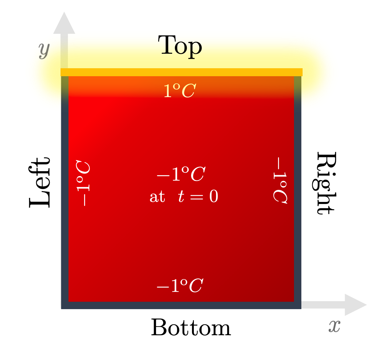
Fig. 1: The boundary and initial conditions used throughout the Heat series. Energy is pumped from the top edge onto an initially completely cold 2D plate. Credits: David Carvalho / Inductiva.

Classical Numerical Methods

As usual, finding governing equations from first principles is actually the easy part. Rather, solving them presents us major challenges. Why?

Most PDEs do not admit analytical, pen-and-paper solutions. Only a handful of cherry-picked differential operators can give rise to closed-form solutions. Lesson learnt — numerical approximations must be used.

But which ones? In which conditions? For what type of PDE?

These are general and difficult questions to answer. Wildly different methods have been curated by the computationally-inclined in the Mathematical and Physical communities — not as recipes set on stone but rather frameworks prone to constant scrutiny.

Mesh-based methods are traditionally the dominant approaches. The main idea is to discretize the domain of interest into a set of mesh points and, with them, approximate the solution. A whole zoo of methods exists, in particular:

• Finite Differences Methods (FDMs) replace the PDE expression with a discretized analogue along a grid with the aid of function differences.

• Finite Elements Methods (FEMs) subdivide the problem domain in multiple elements and apply the equations to each one of them.

• Finite Volume Methods (FVMs) builds a solution approximation based on the exact computation (taking advantage of the divergence theorem) of the average value of the solution function in each of the smaller sub-volumes in which the domain is partitioned.

All these methods have their advantages and shortcomings given the idiosyncrasies of each PDE and setup of the problem. Sometimes they may even coincide — for some simple scenarios (such as regular grids) FEMs and FDMs might end up being the same [1].

Typically, mesh-based classical routines tend to be very efficient in low-dimensional problems on regular geometries. We will then use this convenience to our advantage by applying a FDM in a FTCS (Forward in Time, Centered in Space) scheme.