Finite-Differences#
Authors: Manuel Madeira, David Carvalho
Reviewers: Fábio Cruz, Augusto Peres
Discretizing our domain#
Deciding how to discretize the domain is also far from being set on stone: for a given instantiation of a PDE problem, it is typically one of the most complex steps in its resolution. Squares are cool and all but what if we want to simulate the Heat Equation in a mug or a pan?
We’ll make our lives easier (for now!) by using a regular grid to represent the domain. With the aid of the cube:
in a regular grid with
Consequently, input points
It is in this pixelated world we will express how heat will diffuse away…
From continuous to discrete derivatives#
So, we now need to express a differential operator in a finite, discretized
domain. How exactly do we discretize such abstract objects, like the
(univariate) derivative
or a partial derivative with respect to, say, a coordinate
Being on a grid means that we require information on a finite number of points in the domain. The FDM philosophy is to express (infinitesimal) differentials by (finite) differences between any nodes.
The continuous thus becomes discrete — the differential operator
In essence, we must find an algorithm which can propagate the constrains set by the PDE from the initial conditions as faithfully as possible along the grid. In a more specific sense, you might wonder:
How to approximate
reasonably to obtain for all nodes ?
This is exactly what the FDM solver will accomplish. For that, it has to
approximate the differential operators —
Goodbye operators, hello grids!
Finite Difference Method#
Approximating differentials on a discrete set is also not a recipe set on stone.
Let us look at two Finite Difference approximations to a function of a single
variable
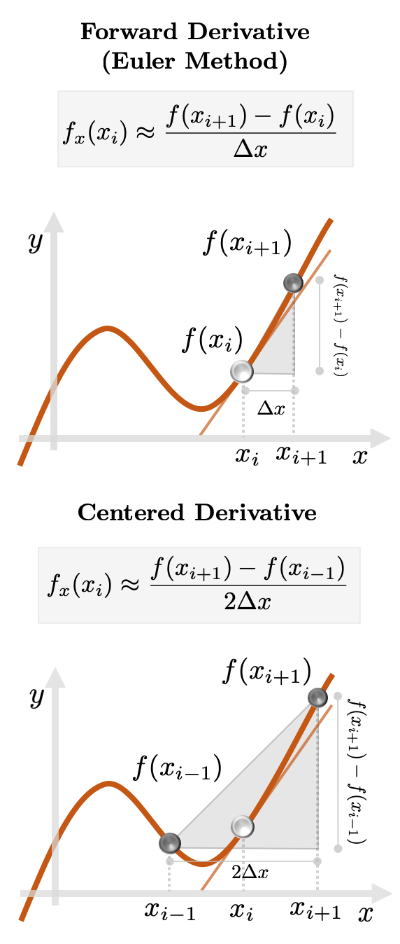
Fig. 2: Approximation schemes of the derivative of
These will estimate the true instantaneous rate via neighboring differences. Expectedly, an error will be incurred in the process.
The price to pay in “dropping” the limit results in a 1st-order approximation,
meaning this estimate scales linearly with the spacing
Choosing how to spread heat#
Given a particular PDE, different FDMs would iterate differently over the grid
node by node to obtain estimates of the differential operators.
So, fixing a scheme is (again) delicate task.
You guessed it right - for this problem, we will use the 2 approximation schemes we showed before to evaluate the differential operators. They are combined in the FTCS scheme:
Forward in Time - the time partial derivative
Centered in Space - the spatial partial derivatives
And then express each first-order term
With a bit of rearranging, both spatial derivatives become:
Look — some terms are evaluated outside the original grid. However, you will notice that these fractional indexes only appear for the computation of intermediary constructions/variables [4].
Heat diffusion on a grid#
Phew! That was intense but we now have all the tools to start simulating heat flow! For that, we must:
discretize the domain by sampling each dimension individually and considering all possible combinations of the coordinates, creating points
discretize the differential operators using a FTCS scheme.
solve for the solution grid
In this fashion, we convert the 2D Heat Equation to this difference equation:
where we can lump all parameters in the ratios:
We can understand how knowledge about the function propagates along the grid with a stencil by depicting which input grid points are needed to iterate the algorithm so a solution estimate may be computed at all grid points.
Fig. 3: A stencil used by the FTCS scheme. At a given node
Credits:
Augusto Peres, Inductiva.
Run our code#
It’s time to play with all these concepts and see how our FDM approximation fares.
All our code can be accessed on our
code snippets GitHub repository.
There, you will find the heat_fdm.py file for simulations and plotting
utilities in /utils.
Have a go yourself!
The role of the
We will pick a spatial discretization of, say,
Fig. 4: Role of various
Heat is on the plate!#
We can reason with these results.
At the beginning (for
From that point on, we can observe the progressive heat diffusion from the hot edge towards lower regions, until we reach a stationary state, where no further changes occur (and the system is in thermal equilibrium).
Heat does not spread evenly across the plate — its spread is faster in regions that are further from the cold regions. Given this symmetric setup, points along the central line between the edges allow for faster diffusion than regions nearby the edges. This will progressively wind down until we reach the cold edges and a paraboloid-like pattern is observed.
But more importantly — the higher the
So — it seems that each internal parameter
Setting stability criteria#
We ran our first PDE classical solver. Yay! However, why are we happy with the results? Clearly, we can think of potential issues, such as:
for excessively sparse discretizations, our approximations of the differential operators will be miserably undersampled and consequently the trial solution will be shockingly wrong.
error buildup will take place as the iterative procedure tends to propagate and amplify errors between any iterations. In those cases, we say that the method is unstable.
However, these are the extreme instances. Were we lucky? If we are using “reasonable” discretizations, a question should make you scratch your head:
How to be sure a certain discretization provides a trustful approximation to the PDE solution?
Fortunately for us, you can notice that the discretization setup can be
monitored exclusively through the ratios
Can we somehow fine-tune them to ensure stability i.e. find admissible combinations of
for a fixed ?
Well, theoretical studies can be performed to find a restricted space of acceptable discretization setups. For our case [3], Von-Neumann analysis establishes a surprisingly simple stability criterion:
These two constants provide a straightforward procedure to be sure that we i) are not oversampling or undersampling a dimension with respect to any other and ii) have spacings that can capture meaningful changes of the solution.
This is not a loose condition.
Just to show you that we’re playing with fire, we cannot think of a more illustrative
example than by ramping up that bound by a mere
Fig. 5: In a discretization step for which
Yup: for this setup, an “explosion” caused by the FDM instability can be seen propagating along the trial solution — quickly unfolding to some psychedelic burst!
At the very beginning, some similarities to the downwards diffusion pattern ( that we just saw previously) quickly fade away as the error buildup spreads away and faster in regions with already large errors.
It’s a race for disaster: the exponential buildup of the errors, even if
sustained for only a handful of propagation steps, ensures that some nodes will
experience huge growth (and NaN (Not a Number). You can see
that eventually all points are not even represented on the scale (they’re
white)!
By the same token, let’s now see what happens if we’re close to the edge from
within the admissible area. Dropping our bound by
Fig. 6: With our parameters recalibrated, stability has been restored! Credits: Manuel Madeira / Inductiva
Incredible! Not even a minimal sign of instability coming through.
We’re happy - we obtained seemingly satisfactory outputs in a reasonable way.
The simulations take about
But remember though: this is an extremely simple system… We could be considering this problem in 3D or at way more complex domains and boundaries. In an extreme limit, we could be using these FDMs in highly-nonlinear equations with hundreds of variables.
To Vectorize or Not To Vectorize – that is not the question#
Understandingly, instructing how to compute many functions over a grid is not a trivial task — issues like computation power and memory storage can be bottlenecks already for discretization setups far from ideal.
We must understand how our implementation choices affect the algorithm performance and the output accuracy. In essence:
How much faster can we solve the PDE without compromising the output?
Using the running time as a metric, we’ll compare 3 mainstream implementations:
Nested
ForCycles: we fill in the entries for the plate at the new time frameForcycles that iterate through theVectorized approach: we perform arithmetic operations on
Compiled approach: we can compile a vectorized approach, which allows sequences of operations to be optimized together and run at once. The code compilation was performed through JAX, using its just-in-time (JIT) compilation decorator.
The approach used is passed as a flag: --vectorization_strategy=my_strategy.
The default is set to numpy and the vectorized approach is used. When set to jax,
a compiled version of the vectorized approach is used and, when set to serial,
the nested For cycles approach is used.
After running each implementation for the same parameters, we obtain wildly different running times:
vectorization_strategy=serial - Time spent in FDM: 93.7518858909607s
vectorization_strategy=numpy - Time spent in FDM: 0.6520950794219971s
vectorization_strategy=jax - Time spent in FDM: 0.297029972076416s
Wow! By using the vectorized approach, we obtain more than a
This is not surprising. The vectorized approach takes advantage SIMD (Single Instruction, Multiple Data) computations, where one instruction carries out the same operation on a number of operands in parallel.
This discrepancy is then easy to understand and a huge acceleration is observed,
in constrast when ran with the nested For cycles, where each instruction is
executed one at a time.
We are not done yet. By compiling the vectorized approach, we obtain yet another
Computation resources are finite (and costly). Despite the huge boost granted by the compiled vectorized approach, this methodology improved our task by 2 orders of magnitude. Is that enough when dealing with far more complex PDEs in higher dimensions?
How far can we push classical methods?#
Despite our pleasant experience with a low-dimensional problem on a regular geometry, we should be careful thinking ahead. Classical methods for solving PDEs have long been recognized for suffering from some significant drawbacks and we will comment on a few:
Meshing#
Meshing becomes a daunting task in more complex geometries. Different discretization setups can always be chosen but once one is fixed, we have limited ourselves to computations on the nodes generated by that particular setup. We can no longer apply arbitrary smaller steps to approximate the differential operators.
Worse still — depending on the behavior of the differential operator, we might need to focus on certain regions more than others. It’s unclear how these choices impact the quality of the approximations.
Discretizing the problem also creates a bias in favor of the grid points with respect to all others.
But what if there the PDE behaves differently outside the mesh?
The best we can do is to infer a solution through interpolation but this is admittedly unsatisfactory.
Scaling#
Classical algorithms scale terribly with the PDE dimensions and grid refinements.
For all the Complexity lovers out there — you know that sweeping the regular
grid
By simply refining our grid by
Similar bad news are expected as we consider simulations on PDEs for higher
dimensions. For a problem of 3D heat diffusion, the complexity grows as
Feasibility#
Even though we can rely on stability conditions, this does not mean we can deploy them — it may be computationally very, very, …, heavy or simply impossible.
As we saw, simulating a medium with higher
This comes at a bitter price and is a major drawback of the FDM.
Machine Learning?#
PDE simulations must be as fast and light as possible. But can classical methods, in general, get fast enough?
We can look farther ahead. Consider something extreme (but likely). Imagine our task is to find parameters that lead to optimal performance for some problem.
Let us assume we have access to the theoretically fastest PDE classical solver, foolproof to instabilities and extremely efficient in terms of memory and processing.
If hundreds, millions, …, billions of intermediate PDE calculations had to be performed with that algorithm, could we afford the computational budget? Would the time elapsed be reasonable?
Certainly not. It is not difficult to estimate runtimes comparable to our lifetime (run across millions of processors!) to achieve some real-life optimization tasks.
This would forbid us from iterating across the parameter space fast enough — Game over.
Efficiency in classical methods won’t provide the scaling we need to
overcome this barrier.
A new paradigm is needed.
Fortunately, a large class of algorithms can handle this curse of
dimensionality exceptionally well. Can you guess what we are talking about?
Yup, Deep Learning!
In the following posts of this series, we will address how we can leverage on those approaches to possibly overcome these issues raised by classical methods.
Until then, don’t melt away!
References & Remarks#
[1]
More on this FEM and FDM possible similarity here.
[2].
The FDM-based approach we present is loosely following this excellent example that
inspired us.
[3].
More details of the derivation of this expression can be found here (pages
11/12).
[4] There are more complex cases where it is convenient to define such staggered
grids with fractional offsets to the original (e.g for Maxwell’s Equations).