Physics-Informed Neural Network#
Authors: Manuel Madeira, David Carvalho
Reviewers: Fábio Cruz
As our scientific and technological needs evolve, it is not unrealistic to expect problems depending on solving billions of partial differential equations (PDEs) with hundreds of variables and defined on high-dimensional spaces with hard boundaries constraints.
Can Deep Learning lend us a hand in this regard? Let’s find out!
Employing a disruptive ethos, in this post we will hopefully convince you that there is a whole lot of potential stemming from Deep Learning (DL) methods in tackling this issue.
In recent years, huge developments in Machine Learning have been triggered by ever-enhancing computational infrastructure and modeling sophistication.
In fields such as Computer Vision or Natural Language Processing, Deep Learning (the sub-field of Machine Learning that handles Neural Networks (NNs)) has evolved as to allow for huge advances in what can be done.
In fact, three extremely powerful points assure any researcher that NNs can be leveraged in their field:
the capability NNs have to succeed handling extremely high-dimensional spaces (for which we have motivated bottleneck-level issues due to the curse of dimensionality will almost invariably arise);
theoretical guarantees of success, namely due to the Universal Approximation Theorem [1];
better still, all the DL software artillery available has dramatically lowered the entry barrier for deploying NNs frameworks. It has never been this easy to set up sophisticated models with a handful of lines of code!
It is no surprise that NNs started invading other territories and Fundamental Sciences are no exception.
Deep Learning for… Partial Differential Equations?#
The underlying laws behind most natural sciences rely on equations dictating how certain quantities vary in time and space. Naturally, we must wonder:
Can we possibly solve such an abstract problem like a Partial Differential Equation (PDE) with the aid of NNs?
To answer this question, let’s first formalize a bit. In PDEs, the unknowns are functions which depend on various variables and are defined over some domain. Solving the PDE (or systems thereof) entails finding such functions.
For a single real-valued PDE with
where
Our hope is thus to find a NN whose output trial solution can mimic the actual PDE solution.
Deep Advantages#
Guess what? As parametric function approximators, NNs are particularly well tailored for this problem.
If you recall what we discussed, many limiting issues are found when numerically solving a PDE via a classical method by discretizing the domain — usually performed with Finite Difference or Finite Element Methods. Ideally, we would like to circumvent these problems.
As we will soon see, PINNs (Physics-Informed Neural Networks) address most of the previously mentioned limitations of the classical methods:
they are mesh-free, making the interpolation for non-mesh points no longer a concern. Once trained, PINNs can be evaluated at any point of the domain of interest. The way the training is performed can also be adjusted so that the function-valued solution we seek can be found in very efficient ways;
there is no such thing as error buildup or instability coming from the iterative nature and discretization imposed by the classical methods.
For now, it’s clear — we should express a solution of the PDE as a NN.
Buckle yourself up and let the fun begin!
Physics-Informed Neural Networks (PINNs)#
We will showcase you one of the hottest approaches to tackle PDEs from a DL perspective — Physics-Informed Neural Networks (PINNs) [2,3].
In what way does this architecture differ from more conventional NN models? Well, firstly we:
try to approximate the function solution to the PDE through a NN that fits some data points that are provided. Typically, these are points set by boundary and initial conditions but they can also be in the interior of the domain;
constrain the space of functions from which the NN can learn by penalizing solutions whose partial derivatives do not satisfy the desired PDE.
The first point is commonplace in DL approaches. This simply entails a ‘supervised’ minimization procedure between the output and the ground truth set by the conditions. This flavor of architecture is normally termed vanilla.
The whole novelty and potential of PINNs stem from the second term, which is the one that fundamentally deviates from the vanilla DL by regularizing NN guesses.
It’s this aspect that coins these NNs as Physics-informed: from all the NNs that we could learn, we are imposing an inductive bias towards those that verify the Physics of the system at hand (i.e. what the conditions expressed in the PDE enforce).
The idea of Physics here is a bit misleading. PINNs do not have to pertain to physical systems. By Physics, it is assumed that some strong principle or law must be held across the system. Curiously enough, these tend to be expressed precisely with PDEs!
Training the PINN#
But how can we obtain a NN that we are confident has mimicked the actual solution of the PDE taking into consideration the two aforementioned notions?
Needless to say, there are many answers, depending on the problem at hand. For instance, we could
try to construct (activation) functions that necessarily respect the differential equation;
if, say, the PDE were linear, use linear combinations of solutions so to respect the PDE;
work in the spectral (frequency) domain — where the derivatives could be tight by some relation — and consequently an inverse fast Fourier transform could be used to map the solution to the direct domain.
A Clever Loss Function#
The answer that requires minimal change though is to tweak the way the loss
function is computed. This objective function
We want to make the loss as small as possible. Once we’re in that regime, we can be fairly sure our trial output is somehow close to the true solution and we can say our model has learnt how to solve the PDE.
Tracking the behavior of
Considering this motivation — admittedly more mathematical — we can now formulate the impact of each term on the overall loss through an individual term:
Output values loss
where
Typically, the
PDE “Regularization”
Easier said than done. This is a colossal task for each parameter instantiation of our NN (hundreds of billions of parameters may have to be recalibrated!)
However, we can benefit from the auto-differentiation artillery that has been developed for NNs: the available packages allow for a straightforward and efficient way of obtaining the partial derivatives with respect to the many model inputs.
In contrast to the first point, this loss term can be applied to any point, given that we do not require prescribed target values.
We are now in conditions to obtain a total loss term by summing both loss terms:
Even though both terms were weighted evenly, this is not a requirement. Actually, it is quite common to find this loss defined as a convex combination of those two terms, where the weighting coefficient is an extra hyperparameter requiring appropriate fine-tuning.
But putting these and other technicalities aside, this is pretty much what you need to know about PINNs to follow the rest of this post!
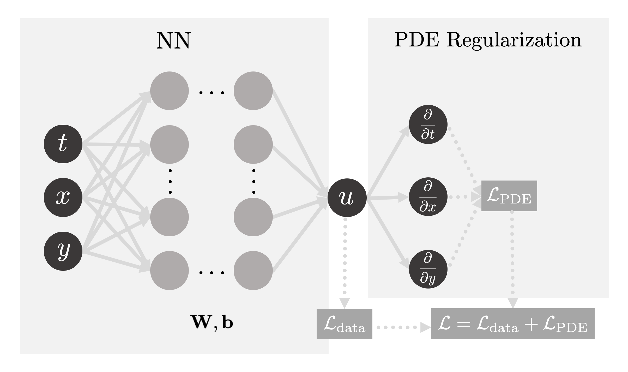
Fig. 1: The PINN we used to solve the 2D Heat Equation consists of two parts:
firstly, by updating the NN’s weights
IDRLnet: a PINNs library#
To set a DL algorithm, we use IDRLnet, a PINNs library built on Pytorch [4]. To the best of our knowledge, it is one of the most versatile open-source PINNs library.
The IDRLnet library has an architecture based on three different types of nodes:
DataNodes- these are essentially domains that are obtained from Geometric Objects (also provided by the library), from where it is possible to sample the points used to train the PINN;NetNodes- these are abstracted from neural networks, i.e. the architecture, training hyperparameters, and everything else related to the NN used are defined in this node;PDENodes- these contain all the information related to the PDE we wish to solve. Contrarily to NetNodes, PDENodes do not have trainable parameters.
Fine — we are ready to try it out on our new favorite PDE: the 2D Heat Equation!
Hot NN Coming Through!#
To keep things simple, let us start with the exact same situation as the one presented for FDM:
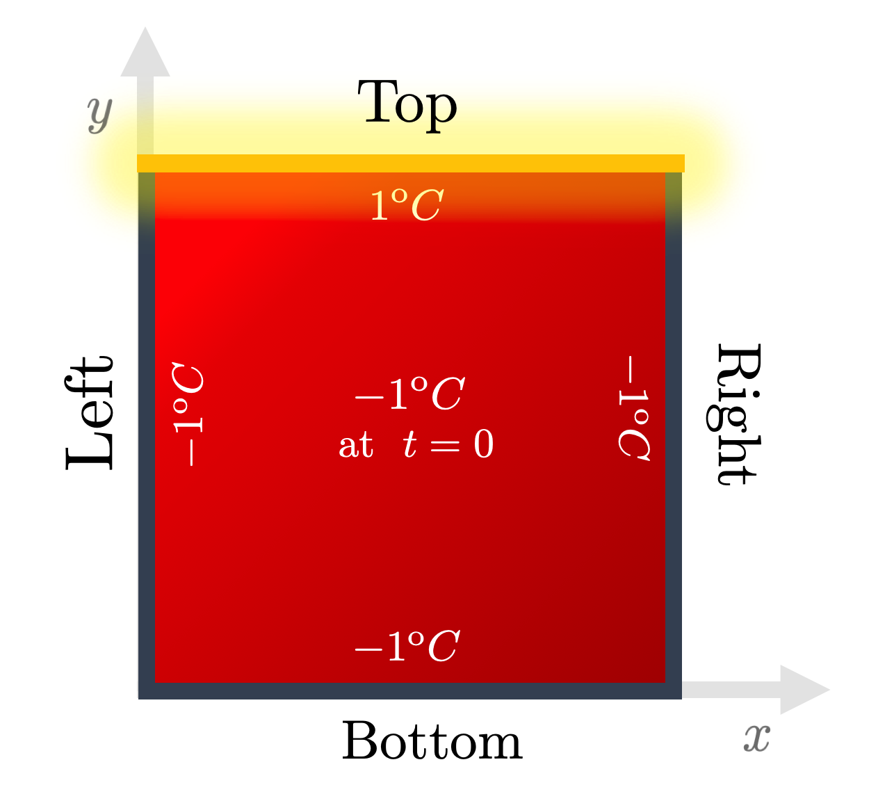
Fig. 2: The boundary and initial conditions used throughout the Heat series. Energy is pumped from the top edge onto an initially completely cold 2D plate. Credits: David Carvalho / Inductiva.
A very simple domain was chosen — a regular 2D square plate. We must then
consider points of the form
Recall that the hot edge was kept at the maximal temperature
(
This prescription allows us to compute the loss term
Time to Heat [Start]#
You can find our code here and run your very first PINN! Run this experiment through the following instruction in the command line:
python heat_idrlnet.py --max_iter=10000 --output_num_x=500 --output_num_y=500 --colorbar_limits=-1.5,1.5
The flags used trigger the following instructions:
max_iterdefines the total number of training epochs;output_num_xandoutput_num_ydefine the discretization along the x-axis and y-axis, respectively, of the grid in which we infer results;colorbar_limitsdefines the range of the colorbar used.
For illustrative purposes, we set the diffusivity constant to
Disclaimer: our code is able to accommodate some extra complexity that is not needed in this post. For now though, we will not dive in detail but let the magic happen in the next section 😎.
Classical vs NN — the fight begins#
To see how well our NN-based framework handles the task, we can compare the NN output to the one generated from the classical Finite-Differences algorithm:
Let’s plot the output obtained with the FDM (a classical algorithm) [top] and a
PINN we trained [middle], as well as the error
heat_error.py python script.
Fig. 3: Comparison of the results obtained via a classical algorithm (a FDM)[top], a DL algorithm (the PINN computed with IDRLnet)[middle] and the absolute value of their difference [bottom]. They seem very similar! Indeed, an inspection of the error shows global convergence. Credits: Manuel Madeira / Inductiva
Wow — this looks rather good!
The NN output approximates quite closely the results obtained with FDM. There are some deviations mainly in the initial instants and then in the upper corners. Actually, these are the regions where sharper transitions of the solution function are found, and it is thus natural that our PINN has more difficulty to fit correctly there.
This certainly seems hopeful — but an inquisitive mind like yours must be wondering about why this PINN worked.
How long should we train?#
In order to train the PINN, a rather large number of epochs
(
This can make us think: just like the classical algorithm had to be tuned so no nonsensical estimates were output, there must be some suitable tuning to assure us the algorithm can indeed approximate the solution.
Fig. 4: Difference between the PINN output after training with different number
of epochs and its respective classical output (serving as a benchmark). We can
see a substantial error for few epochs (
The results are just as we expected: the higher
Specific knowledge of the PDE or domain in question may make our lives easier!…
Customized training#
The versatility of the PINNs in focusing on different regions differently begs a question of the utmost relevance:
Are we favoring or penalizing regions that require a different level of refinement?
Fortunately, via TensorBoard, it is possible to track various loss terms throughout the training procedure by using the command
tensorboard --logdir [insert path to "network_dir"]
With it, we can then see the effect of extending the training procedure. For this, we set different numbers of epochs and see how the output is impacted by this choice.
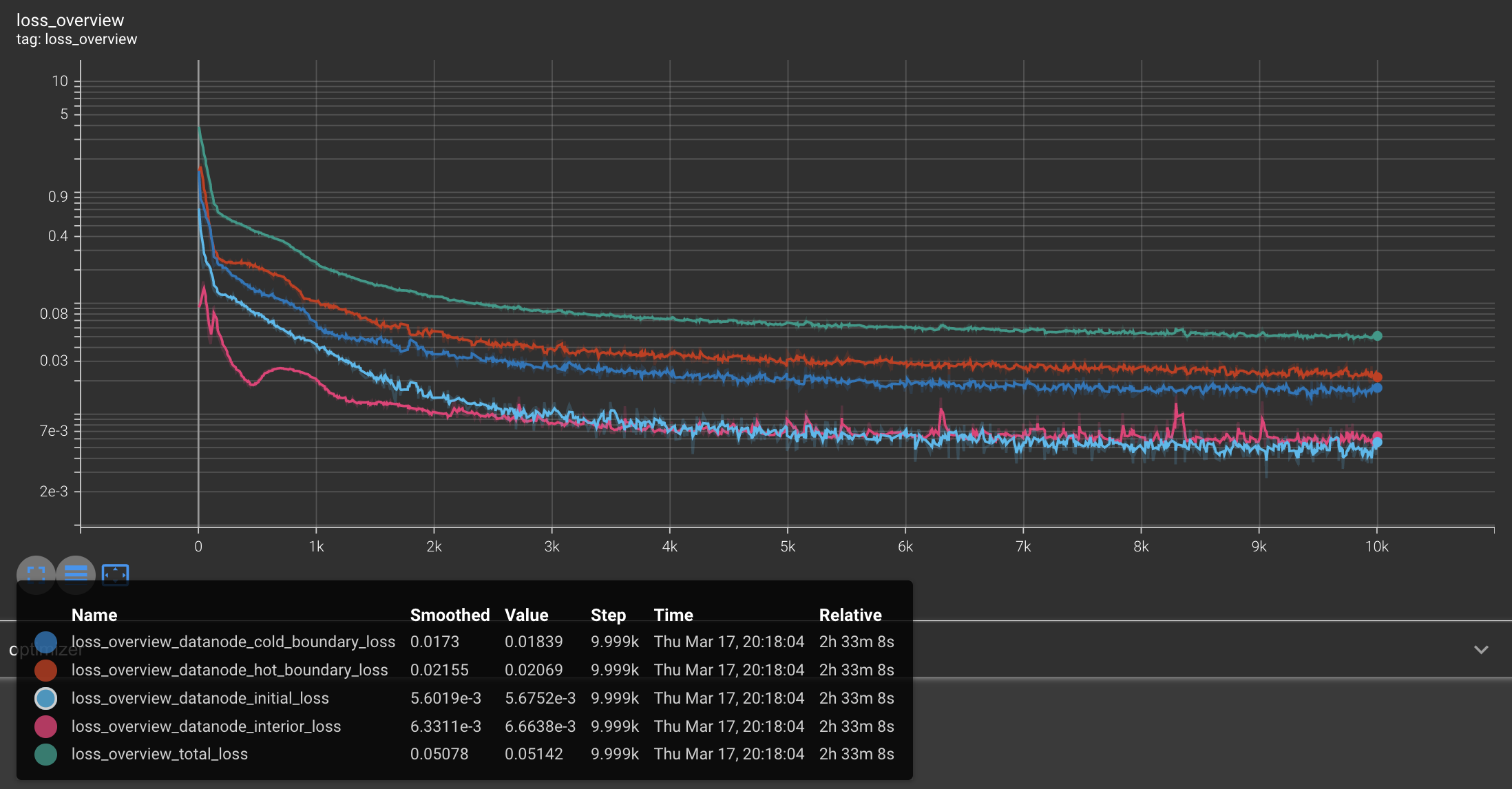
Fig. 5: Learning curves (in logarithmic scale) for different sub-domains. We can see that, even though all terms have different behavior, they eventually converge to exceedingly small values. Credits: Manuel Madeira / Inductiva.
You can see how the loss for various subdomains (the captions should be clear to follow) changes as training takes place.
The training of PINNs (or generally with NNs), is not a completely trivial task. In fact, from the learning curves above, it is clear that if we stopped our training too early on, our results would be necessarily worse.
The ghost of overfitting#
We typically find overfitting whenever we train our model excessively with a training dataset — ultimately providing a strict fitting across the given data points, or when training using a closed dataset (by not using randomly-generated data).
This leads to a huge drawback: the model loses its generalization capability.
In other words, when we present the model to new unseen data still from the same distribution that generated the training dataset, the model will have weak predicting power for those points and thus a much higher loss rate.
A validation set of data points is typically kept in parallel to the NN training procedure to ensure, through periodic checks, that we do not enter such an overfitting regime.
In this case, we do not have to worry about the possibility of overfitting for two main reasons:
firstly, we are sampling a different set of data points in each epoch, i.e., our training set is changing from epoch to epoch
secondly, we are considering a regularization term in our loss (recall
Furthermore, we see that points coming from the boundary conditions are the most troublesome ones — due to their higher loss. To contrast this, FDM implementations have those points directly hard-coded onto the final solution.
Learning Rate#
Another typical issue impacting the performance of PINNs (and NNs in general) is
the choice of the learning rate
This is a hyperparameter — a variable which pertains to the structure of the model itself. The update of the NNs parameters is performed by applying optimization algorithms, thus known as optimizers.
The way in which the learning rate is exploited in these optimizers varies. However, we can intuitively think about it as the magnitude of the step given in the parameters space in each iteration.
Striking a balance between speed and accuracy is not only a vital part of setting the model but also a delicate task on its own.
A larger learning rate allows us to have larger updates in the parameters and thus faster progress but at the same time it may lead to large instabilities in the convergence process. In extreme instances, we may never be in conditions to access the optimal regions.
To see this, let us see the effect of using larger and smaller learning rates
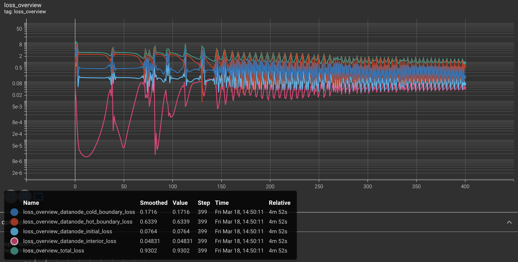
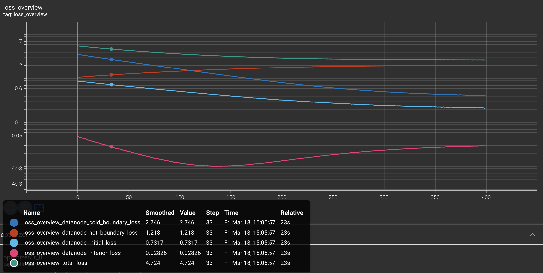
Fig. 6: Learning curves (in logarithmic scale) for two different learning rates.
Note that a very large rate
On the one hand, for
Contrary to this regime, a small rate
Balancing performance, accuracy and computation resources surely is a sophisticated feat!
There is art in DL#
The lesson we learnt here is that indeed NNs can be adequately trained to yield estimates of PDE solutions without explicit computation of the PDE.
For that though, we must be crafty — choices like the learning rate and the number of epochs directly impact the performance of the PINN.
The fine-tuning of hyperparameters is not something set on stone and requires subtlety and exploration to be successful. The technical aspects and their formulation are still open topics and intensively studied in the DL+ML communities.
Just as with FDMs we had to fine-tune the discretization parameters in order to ensure the stability of the method, the same must be considered for PINNs — they are not a panacea! Even though it offers an edge in streamlining the computation of the estimate, extra care is still needed!
NN architectures come in many flavors and recipes and may be improved in many intuitive ways. As a general question, we can wonder:
Should we take some inspiration from the classical methods and explore a direction where the boundary (and initial) conditions are hard-constrained in the learning problem (e.g. verified by construction)?
This is one of the questions that we are tackling at Inductiva — and we will show you more as progress is made 😛!
Next episode#
In the next (and final!) section of our tutorial, we will precisely unveil some of the aspects that can make our problem harder to solve but also more realistic.
In particular, we will show you how to extend this vanilla version of PINNs to be able to:
deal with complex geometries (rather than a simple square plate);
solve a PDE to more than one instance of the boundary conditions without having to retrain the whole model again.
Neural Networks sure sound exciting, right? Stay tuned 🌶️!
References#
[1] A bit more
about the mathematical foundation for the suitabillity of NNs to model
challenging maps from input to output.
[2] Defining papers outlining the architecture
and ideas of PINNs in the Literature.
[3] Yet
another influential paper on PINNs.
[4] Check out the documentation of the
IDRLnet library here.