Generalized Neuro-Solver#
Authors: Manuel Madeira, David Carvalho
Reviewers: Fábio Cruz
In this section, we are going to show you that a grand unification of gravity within a quantum field theory framework can explain topologically nontrivial dynamics observed in simulations of graviton inelastic collisions in a AdS space. Let’s go!

It’s all good. We’re just messing with your mental sanity!
Ok. Now that we have caught your attention, let us snap back to reality — maybe one day we will pay this topic some attention!
Even though we won’t achieve such an ambitious goal as the one mentioned above, in this final post of the Heat series, we are going to fulfill our overarching promise:
to showcase the strength and versatility of Neural Networks (NNs) in solving hard Partial Differential Equations (PDEs) in challenging domains and conditions.
In this final instalment of the Heat series, we delve once more into this topic with the aid of our very cherished Heat Equation. So let’s go!
Introduction#
So far in this series, we showcased a classical algorithm and a Neural Network
(NN) to solve the Heat equation. Both of these implementations were performed on
an extremely simplistic (and unrealistic) scenario.
It is as straightforward as it can get:
the heat equation is a linear PDE: the solution function and all its partial derivatives occur linearly, without any cross products or powers and any spacial preference for any of the (only) two coordinates. This form of PDE is one of the simplest we can face.
a very idealized medium with a constant diffusivity
very simplistic conditions: the geometry considered of a square plate where the boundaries are always kept fixed and the heat flow uniformly set up along the upper boundary is quite utopian in practice. Real-life plates have deformities, changes in density, imperfections…
So, we ought to ask the question:
How can we strengthen our case — that NNs can handle more complex and nontrivial cases?
This is exactly what we want to address. We will ramp up the complexity of these scenarios and see how well NNs can potentially fare.
This won’t be done with much sophistication — the approach we adopt is very incremental and straightforward. Most importantly though, it serves the purpose of a simple demonstration of the principle of generalizing learning algorithms.
Rethinking the NN architecture#
Ok. What do we mean by generalization power?
Think of a PDE — apart from the structure of the differential operators acting on the solution, there are many other variations that can impact its behavior: internal parameters (such as physical properties) but also the initial and boundary conditions (IBCs).
Getting a NN to learn for a particular instantiation of these conditions is hard on its own. We could naively consider adding extra dimensions and run a NN that would be trained point by point by grid-searching on yet a bigger space.
This surely does not sound scalable. If we want to see the effect obtained
from ever-so-slightly different conditions on the same PDE, we have to rerun the
whole classical method or perform the entire NN training task again.
This is highly unsatisfactory!
Worse still: the required time to train the PINN increases rather substantially. Generalization power requires heavy computational resources and routines that must handle the completion of the algorithm efficiently. In either case, the training time naturally becomes a major bottleneck.
How to tackle these issues?
Hard-(en)coding the variability#
There are two direct answers — either we directly:
decrease the training time by exploiting some magically-enhanced novel procedure which can accelerate the PINN’s weights and biases fitting somehow. As we discussed before, this seems quite unlikely and it is unclear if this factor could counteract the scaling effects.
increase the yield from that training process: what if, for the same effort in training, we could obtain better predictions or cover a larger set of physical cases?
It is from the second direction that the generalization idea comes out. Given that we will have to train our PINN anyway,
why don’t we try to make it learn the solution function for different sets of internal or external factors from the get-go?
We can do this by hard-coding the prescription of conditions or parameters by including appropriate representations in input space directly in the model. Only then we can say the model has a shot at learning for generalized cases.
But this isn’t trivial by itself. Imagine you want to use a vanilla NN in a supervised way. To train it, you would need a ground truth given by say, a classical algorithm. Each such process would have to rerun for each new set of parameters or conditions. This can take a lot of time.
On top of that, how to know which conditions to sample from? Depending on the quality of the sampling used to generate the ground truth (in this case given by a classical simulation algorithm), the model can now in principle be used as an oracle which, if well trained, will return confident outputs for unseen parameters. But we now know sampling the phase space can be extremely slow or downright unfeasible in this setting. So we may wonder:
But what if we don’t need a ground truth at all in our NN?
Well, we would bypass the need to run expensive and heavy classical algorithms!
Granted, constructing efficient neuro-solvers is far from trivial. However, the upshot of such hard and laborious work to get the model to learn the generalized task can be huge — a considerable advantage in favor of NNs, as their inference can be significantly faster than classical methods.
If NNs succeed in this task, they can potentially solve PDEs in theoretically all possible conditions! In this perspective, NNs supersede “grid-like” algorithms where adding such parameters results in an exponential curse of dimensionality.
It sounds powerful, right?
Now, let’s get things on more concrete ground… You know the drill: it’s time to get hot in here!
A neuro-solver for the Heat Equation#
We have been advertising PINNs (Physics-Informed Neural Networks) for their flexibility as a DL framework, so you guessed it right — we are going to use them to showcase how generalizational power can be harvested from picking appropriate algorithms that can handle such beasts as dem’ mighty PDEs!
To test these notions of generalization, we will consider our usual setup of heat diffusion across a 2D rectangular plate:
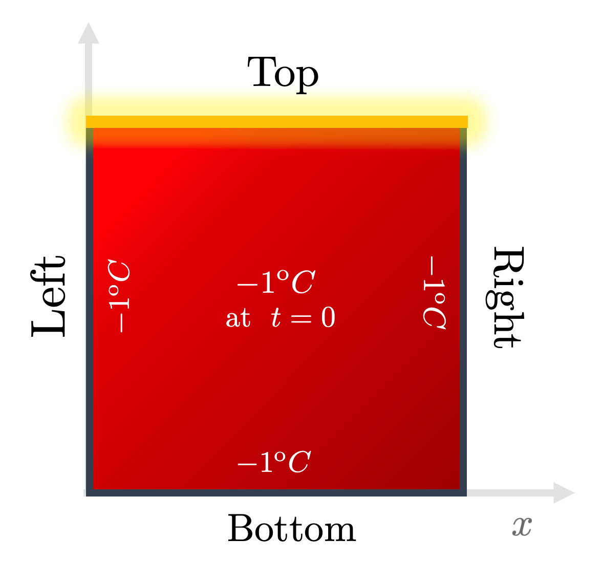
Fig. 1: The usual initial and boundary conditions (IBCs) we assume to solve the Heat Equation on the 2D plate. Credits: David Carvalho / Inductiva.
It states that the temperature profile
With it, let’s investigate three topics:
Learning for parametrized boundary conditions: keeping this admittedly simple domain, we parametrize the top edge temperature
Learning for different domains: we see how well PINNs can solve when using more complex geometries. We will solve the Heat Equation with a PINN in a more challenging domain, where a spherical hole is punched into the interior of the plate.
Learning without generalizing: we will benchmark how much slower it gets if generalization principles are neglected. In other words, we will adress generalization by brute force. Using our new holed plate, we will run PINNs that can solve across this harder domain when trained (each at a time) for various diffusitivities
Let’s Heat run#
You don’t need to program anything — you can find and run our code in our
dedicated github repository
here and train your powerful
PINNs!
Getting a PINN to generalize across boundary conditions#
Until now, only fixed scenarios for which the boundary and initial conditions were set a priori were used (like the ones just above). In this framework, the PINN is trained to fit exclusively with those conditions.
This is naturally far from ideal. If we were to change the initial temperature of any edge by a teeny tiny bit, the model output for such a system would already be of dubious predictive power!
So, we face a structural question here:
How can we encode this boundary information as input to the PINN in a way the model can effectively generalize its effect on the output solution?
To answer this, let’s focus on an extremely simple setup to showcase this training capability. We will keep all boundary and initial conditions fixed except for the temperature of the top edge, which can now change.
Once again, we pick the simplest approach to achieve generalization: via parametrization. In this way, we think of encoding the variation by means of variables (or any other sensible descriptor) to allow the NN to extend the solution function to other IBCs natively in its architecture.
In this simple configuration, a single parameter
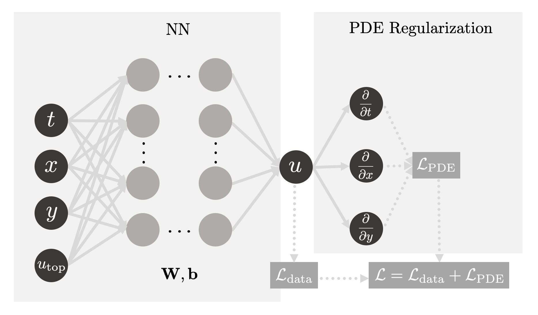
Fig 2: Our PINN will now be able to learn the behavior of the solution as the
hot edge temperature
To see how well the PINN fares, we:
train it by sampling many instances of
then infer for the unseen case
Running…#
Do you remember when in we mentioned that our implementation was able to accommodate some extra complexity? Time to exploit it!
The command line instruction to trigger this experiment and generate the PINN output is simply:
python heat_idrlnet.py --max_iter=10000 --output_folder=generalization_bc --hot_edge_temp_range=-1,1 --hot_edge_temp_to_plot=0 --output_num_x=500 --output_num_y=500 --colorbar_limits=-1.2,1.2
The script heat_idrlnet.py trains a PINN in the setting described throughout
the Heat series. The flags in this command line fulfill different purposes:
max_iterdefines the total number of training epochs;output_folderdetermines the directory where the resulting files stemming from the PINN training procedure are stored;hot_edge_temp_rangeis the range of hot edge temperatures within which the PINN is trained;hot_edge_temp_to_plotis the hot edge temperature to which we intend to infer results;output_num_xandoutput_num_ydefine the discretization along the x-axis and y-axis, respectively, of the grid in which we infer results;colorbar_limitsdefines the range of the colorbar used.
Let’s analyze it by using a classical Finite Difference Method (FDM) for
Fig. 3: A PINN estimate of the solution of the Heat Equation for a top edge
temperature
Very nice! As expected, the network [top] recovers the diffusion patterns
predicted by the classical algorithm [middle]. We can track the error by
plotting their difference [bottom], where a great resemblance arises. This plot
can be easily obtained by running the provided heat_error.py python script. We
notice that the main source of error is found in the upper corners where cold
and hot edges get in touch, generating an extremely sharp transition that the
PINN struggles to keep up with.
Even though some minor numerical deviations are seen, these are justifiable given that the task that we have provided to the PINN is significantly harder, and we kept the total number of epochs and Neural Network architecture as before in the series.
Lesson: for the same amount of training, clever architectures can indeed provide us the generalization power we sought, saving us a huge amount of computation resources and with very little damage in results accuracy!
Probing complex geometries#
We are interested in testing PINNs for more complex geometries than the regular square plate. Let us then now go the extra mile and address precisely the challenges of probing different domains with NNs.
PINNs are particularly well suited to address complex geometries as it only requires a proper domain sampler that provides both:
boundary and initial points with the correct target value (given by the ground truth);
and interior points where the PINN computes the PDE residual and then backpropagates it.
In fact, the PINN solution function will be defined for values outside of the domain considered, but we just neglect it.
Our code implementation supports designing a plate with an arbitrary number of holes inside the problem domain. Let’s focus on a single hole at the plate center:
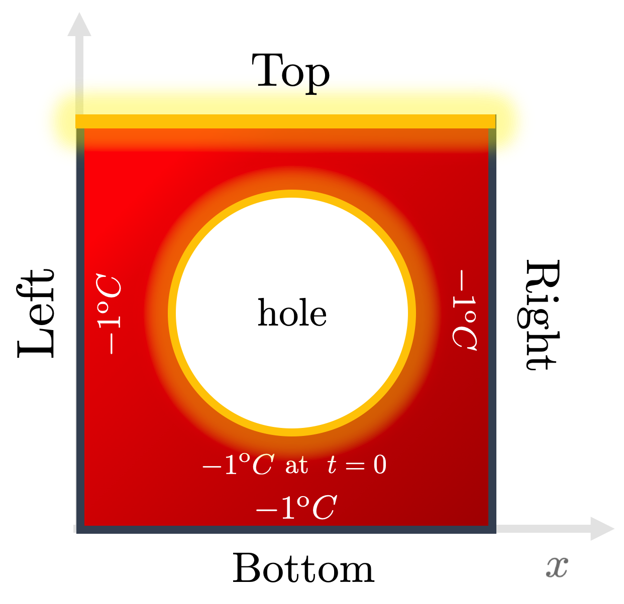
Fig. 4: We now generalize our boundary and initial conditions given the domain
by taking the top edge temperature as a variable parameter
Given this, we keep the boundary and initial conditions as in the previous
setting (top edge at the maximal temperature (
We consider two types of holes now:
Hot hole: The points sampled from the hole boundary are set to the maximal temperature (
Cold hole: Conversely, in this case, the points sampled from the hole boundary are set to the minimal temperature (
Running our code#
Let’s now get some code running! The instruction in the command line that leads to the PINN results is the following:
python heat_idrlnet.py --max_iter=10000 --output_folder=hot_hole --holes_list=0,0,0.1 --output_num_x=500 --output_num_y=500 --colorbar_limits=-1.5,1.5
For instance, the cold hole setting can be run as:
python heat_idrlnet.py --max_iter=10000 --output_folder=cold_hole --holes_list=0,0,0.1 --holes_temp=-1 --output_num_x=500 --output_num_y=500 --colorbar_limits=-1.5,1.5
Regarding the new flags in these command lines:
holes_listis the list of holes we consider in our plate, where each group of three contiguous entries define a hole asholes_tempdefines the temperature of the holes boundaries (it is not defined for the hot hole as it is
So, for the same
Woah! The results from these experiments are clear: the hole in the domain clearly affects the heat diffusion profile in very different outputs!
When the hole boundary is cold, the heat source remains the same and so the same general downward parabolic-like behavior we’ve discussed is observed. The main difference is that heat flows around the hole.
The more interesting case occurs when we also pump energy into the plate through the hole boundary. In that case, another pattern is added – a radial outflow. The interference between these two streams is obtained in opposite directions: while the cold hole suppresses the heat diffusion towards closer regions to the hole border.
But this is still intuitive enough. But how to think of a highly complex interference pattern? Let’s put our code handling more exotic domains!
For instance, let’s think of more physically-relevant cases. Can we understand the physics behind this irregular setting where 3 holes of various sizes and positions are found and the boundary is now curved?
Fig. 6: Heat flow across a more complex domain composed of three holes of varying sizes and positions, as well as curved left and right boundaries. Credits: Manuel Madeira / Inductiva.
Generalizing through grid-searching (is inefficient)#
To make a point (and get more awesome visualizations 😁), let’s see how the
output changes by changing the diffusitivity rate
For that, we simply run each PDE for each
Fig. 7: Heat diffusion profile in the holed domain by ramping up the
diffusitivity from
Hot! We can see that the diffusitivity allows us to disentangle both phenomena
streams we discussed (downward vs radial). Additionally, it sets the time scale
for equilibration, when the state becomes stationary i.e. whenever
The main point to grab here though is that the output you see comes after training each PINN individually! For instance, for these settings, each PINN will take about 5 hours. This is completely inefficient and does not allow the algorithm to organically understand how to map the IBCs to the output.
The PINN architecture behind generalization#
In order to make generalization tangible, the computing infrastructure needs to be versatile and efficient. From a computational perspective, we should ask:
How exactly does the PINN change to accommodate for this generalization?
The fact that the loss function differs according to the domain from where the data domain points considered are sampled is of huge computational relevance.
While a initial or boundary point is directly fit by the PINN to its target (imposed by the initial or boundary condition itself), a point stemming from an interior domain contributes to the fitting procedure through its PDE residue.
PINNs do not impose an upper limit to the number of IBCs or interior domains. Each of these IBCs may have a different target and each interior domain might be assigned to different PDEs. As you can imagine, for complex problems, PINNs have a high chance of turning into a mess!
Let’s make use of a perk from the IDRLnet library (which supported us throughout
the Heat series) — a visual representation of the computational graph (in
terms of IDRLnet nodes) underneath the implementation it receives.
For this our instance, the representations obtained can be visualized as:
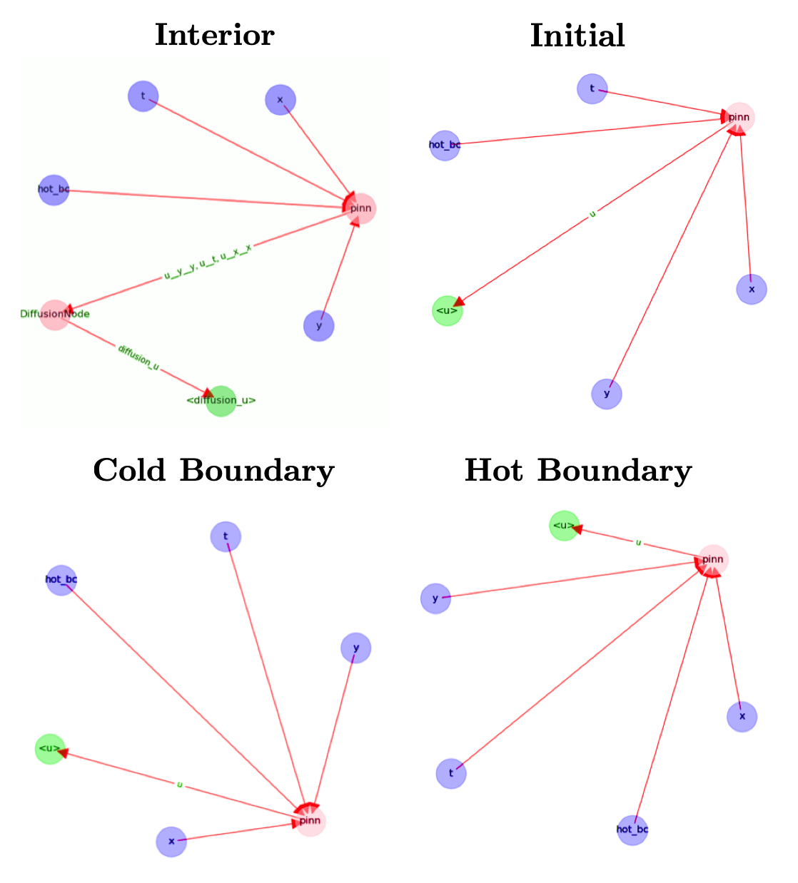
Fig. 8: Computational graphs considered by IDRLnet for each sampling domain considered. If we added holes to our plate, an extra graph would be obtained (similar to the ones from the IBCs). Credits: Manuel Madeira / Inductiva.
Note that the blue nodes are obtained by sampling the different domains considered (DataNodes), the red nodes are computational (PDENodes or NetNodes), and the green nodes are constraints (targets). [2]
Having a graphical representation of what is going on inside our code is always helpful. Naturally, this tool may become extremely handy to ensure that the problem solution is well implemented.
Conclusion#
Well, it has been quite a ride! To finish off the tutorial, we took the opportunity to sail through seas that classical methods can not achieve (or at least through simple procedures). The reason is that they are not scalable with increasing parameter customization. Classical methods have underwhelming potential in providing acceleration into solving PDEs.
We argue Neural Networks have the capability of streamlining these high-dimensional increments by generalizing more smartly. But the complexity has been transferred to other issues. As we alluded before, the choice and fine-tuning of variables and parameters is not something trivial to achieve (either through classical and DL frameworks).
To see how versatile NNs can be, we pushed a little harder and checked if adding more complexity could be coped by Physics-Informed Neural Networks (PINNs). In a modest setup of incremental difficulty, we sure have explored a lot of situations and probed potential means to achieve smarter training.
This strategy of adding new parameters as simple inputs to achieve generalization is the simplest one (but arguably not the most efficient one).
There are several alternatives — a great example is HyperPINNs [1], whose results have been published recently. They result from the fusion of hypernetworks and the more conventional PINNs. Most importantly, HyperPINNs have been shown to succeed in achieving generalization — although in a different implementational flavor.
The outlook message to us is simple to state. The issues pointed out and run experiments illustrate two essential aspects that will need to continue being optimized are different in nature:
the power that Machine/Deep Learning techniques have to propel scientific computing to unseen new paradigms;
the challenges in computation and algorithm architecture caused by evermore realistic and refined systems of interest.
References & Remarks#
[1] A great introduction to HyperPINNs!